Parametric sweep with pympcc.sensitivity

pympcc.sensitivity returns \(\partial x^* / \partial p\) at a converged solution from a single KKT linear solve — much cheaper than re-solving for every \(p\). This notebook validates the linearisation on a parametric MPCC with a strictly complementary optimum.

import warnings
import numpy as np
import jax.numpy as jnp
import matplotlib.pyplot as plt

import pympcc

A parametric MPCC

\[ \min_x \tfrac12 (x_0 - p)^2 + \tfrac12 (x_1 + 1)^2 \quad\text{s.t.}\quad x_0 \ge 0 \perp x_1 \ge 0. \]

For \(p > 0\) the global optimum is \(x^* = (p,\, 0)\) — the \(H\)-active branch — with \(f^* = \tfrac12\). So \(\partial x^* / \partial p = (1, 0)\). Strict complementarity holds: \(G_0 = x_0 = p > 0\), \(H_0 = x_1 = 0\).

def build(p_value):
    return pympcc.MPCCProblem(
        n=2, n_comp=1,
        x0=np.array([max(p_value, 0.1), 0.1]),
        xl=np.zeros(2),
        objective=lambda x: 0.5 * ((x[0] - p_value) ** 2 + (x[1] + 1) ** 2),
        gradient=lambda x: np.array([x[0] - p_value, x[1] + 1.0]),
        comp_G=lambda x: x[0:1],
        comp_G_jacobian=lambda x: np.array([[1.0, 0.0]]),
        comp_H=lambda x: x[1:2],
        comp_H_jacobian=lambda x: np.array([[0.0, 1.0]]),
    )

p0 = 1.5
problem = build(p0)
result = pympcc.solve(problem, strategy="scholtes", tnlp_refine=True)
print(f"x* = {result.x}      (closed form: [{p0}, 0.0])")
print(f"strict complementarity: G={result.G[0]:.4f}, H={result.H[0]:.4f}")

x* = [1.50000000e+00 4.99635364e-09]      (closed form: [1.5, 0.0])
strict complementarity: G=1.5000, H=0.0000

Sensitivity at \(p_0\)

Active rows for this strictly-\(H\)-active problem are reported by active_row_labels:

labels = pympcc.active_row_labels(result, problem)
print("active rows:", labels)

active rows: [('H', 0), ('xL', 1)]

We need:

• dgrad_L_dp — \(\partial(\nabla_x L)/\partial p\). The Lagrangian is \(L = f(x) - \nu^G G(x) - \nu^H H(x)\), and only \(f\) depends on \(p\). With \(\nabla_x f = (x_0 - p,\ x_1 + 1)\), the derivative is \(\partial(\nabla_x L)/\partial p = (-1, 0)\).

• dc_dp — derivative of the active-constraint residual w.r.t. \(p\). Active rows are \(\{H_0\}\), and \(H_0(x) = x_1\) does not depend on \(p\), so dc_dp = 0.

n, n_p = problem.n, 1
dgrad_L_dp = np.array([[-1.0], [0.0]])

n_active = len(labels)
dc_dp = np.zeros((n_active, n_p))   # neither G nor H depends on p

with warnings.catch_warnings():
    warnings.simplefilter("ignore", UserWarning)
    sens = pympcc.sensitivity(result, problem,
                              dgrad_L_dp=dgrad_L_dp, dc_dp=dc_dp)

print("dx*/dp =", sens.dx_dp.flatten())
print("(closed form: [1.0, 0.0])")

dx*/dp = [1. 0.]
(closed form: [1.0, 0.0])

Linearised prediction vs. re-solve

deltas = np.linspace(-0.7, 0.7, 9)
predicted = np.array([result.x + sens.dx_dp.flatten() * d for d in deltas])

resolved = []
with warnings.catch_warnings():
    warnings.simplefilter("ignore", UserWarning)
    for d in deltas:
        r = pympcc.solve(build(p0 + d), strategy="scholtes")
        resolved.append(r.x)
resolved = np.array(resolved)

fig, axes = plt.subplots(1, 2, figsize=(9, 3.2), sharex=True)
for k, ax in zip([0, 1], axes):
    ax.plot(p0 + deltas, predicted[:, k], "o-", label="linearised")
    ax.plot(p0 + deltas, resolved[:, k], "x--", label="re-solved")
    ax.set_xlabel("p")
    ax.set_title(f"$x_{k}^*$ vs. p")
    ax.legend()
fig.tight_layout()

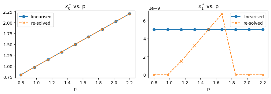
The linearised prediction matches the re-solve exactly along the \(H\)-active branch — that’s the regime where the implicit function theorem applies. Push \(p\) negative enough and the active branch switches (the optimum moves to \(x = (0, -1)\) if you allow \(x_1 < 0\), or to a degenerate biactive point if not); the linearisation then breaks down. pympcc.sensitivity would refuse to extrapolate by returning skipped_reason="biactive_pairs" rather than reporting an unreliable value.